Forecasting with Exponential Smoothing

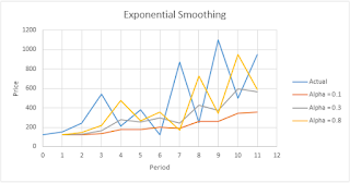
Exponential smoothing  is called the Exponential Smoothing is a method of forecasting the moving average gives more weight exponentially or multilevel on his latest data so that the latest data will get bigger weights.

In other words, the newer or increasingly nowadays, the larger the data anyway does it weigh. This is because the latest data are considered more relevant so that greater weight is given. Parameter smoothing (smoothing) is usually denoted by α (alpha).

Understanding Exponential Smoothing according to experts

The following are some definition or understanding of Exponential Smoothing (Feathered Stratified) according to the experts.

Exponential Smoothing is the technique of moving average forecasting with weighting where data are given more weight by an exponential function. Analysis of the process is one of time series analysis, and is forecasting method with the weighting value on a series of previous observations to predict future values.

It is a type of forecasting technique of moving average that does weighing against past data with exponential way so that the data most recently have weights or larger scales in the moving average.

Forecasting 

Exponential Smoothing Forecasting method or Exponential Smoothing (multilevel Refinement) is widely used to predict the demand for goods (demand) that changes very quickly.

How to Calculate Exponential Smoothing?

With This Forecasting Method  is quite easy, that is by pasting a forecast demand now with the data demand real or actual request data into Exponential Smoothing formula. Here is a formula to calculate it:

Formula 

FT = F_{t – 1} + α (D_t-1 – F_t-1)

Where:

FT = Forecast Demand now
F_t-1 = last demand Forecasting
Exponential Constants α =
D_t-1 = Real Demand

Case Example How to Calculate 

A company that sells its product wants to predict demand Calculator on the market. The method used is the Exponential Smoothing method . The company uses the Constants α = 0.1. Forecast Demand or demand for the month of January is 10,000 units. But in fact, the actual demand in January is only as much as 9,000 units. What is the forecast for the month of February?

Note:

α = 0.1
F_{t – 1} = 10,000 units of
D_{t – 1} = 9,000 units
Ft =?



Answer:

FT = F_{t – 1} + α (D_t-1 – F_t-1)
Ft = 10,000 + 0.1 (9,000 – 10,000)
10,000 Ft = + 0.1 (-1,000)
Ft = 10,000 + (-100)
Ft = 9,900



So the forecast demand for the month of February was 9,900 units.

For Forecasts in the months that followed, we can calculate the same way. Please see the following examples:

The determination of the value of the constant in the Exponential Smoothing Forecasting Method

The value of the constants can be determine by way of trial and error (try). But it can also use the formula below:

α = 2/(n + 1)

Where:

Α = the value of the constant
n = number of periods of time

Example:

If the data consists of 9 months, then α can be obtain by using the following calculation:

A = 2/(n + 1)
α = 2/(9 + 1)
α =
α 2/10 = 0.2

So the value of the constants that we can use is 0.2.